Opening a parachute using Mathematica
One of the classic problems in a first course in differential equations is to model a skydiver jumping out of a plane in the presence of air-resistance. It is good to know how to use software tools to numerically solve these sorts of problems. I recently learned how to do this using Mathematica, which I am excited to share with you.
The setup
Before I use Mathematica to model a skydiver jumping out of a plane and opening their parachute at a specified time \(t_0\), I want to set up the underlying differential equations. One way to think of this is to break it up into two initial value problems. Let \(h(t)\) denote the height of the skydiver above ground as a function of time. If we assume that air-resistance is proportional to velocity, we get the initial value problem \[ \begin{cases} h^{\prime \prime} (t) = -g - r_1 h’(t) \\ h(0) = h_0 \\ h’(0)=0\end{cases}.\] Once we have an explicit solution for \(h(t)\), we have a description of how the skydiver falls before deploying their parachute. We can then compute \(h_1 = h(t_0)\).
I’ll assume that the parachute fully deploys instantaneously (which is a bad assumption, as pointed out by Meade and Struthers), and so we have a new initial value problem \[ \begin{cases} h’‘(t) = -g - r_2 h’(t) \ h(t_0) = h_1 \end{cases}.\]
We can see that the second initial value problem is really the same as the first one except for the parameter \(r_i\) modeling the air-resistance.
This makes it easier to use Mathematica to compute the solution, once we know how to use WhenEvent inside of NDSolve.
The basics of numeric solutions to ODEs in Mathematica
The main command we will use to solve the ODE is NDSolve.
As the name suggests, this solves a differential equation numerically.
he basic syntax is something like
g = 32;
r = 0.15;
h0 = 10000;
eqn = {h''[t] == -g - r*h'[t]}
cond = {h[0] == h0}
NDSolve[{eqn,cond},h,{t,0,10}]
This will return a Mathematica InterpolatingFunction that satisfies the differential equation. One thing I could have done differently is to incorporate the equation and the initial condition into a single list, but when things get more complicated later this helps keep me organized.
How to stop
The last list {t,0,10} tells me that the solution should be valid on the range \(0 \leq t \leq 10\) but we don’t have any guarantees outside of that time range.
One question we might like to answer is “how long do we have until the skydiver hits the ground?” But we can’t really know that until we have the soluition. So my choice of upper bound for the time is really arbitrary.
One way to fix that is to use WhenEvent to tell Mathematica to stop solving the equation as soon as the height is 0. Heres how we do that:
events = {WhenEvent[h[t] <= 0, "StopIntegration"]};
NDSolve[{eqn, cond, events}, h, {t, 0, Infinity}]
Now we will keep trying to solve the equation until the skydiver’s height is 0, and we don’t have to know the upper bound.
Here, setting the upper bound of integration to Infinity is a convenent placeholder for “not knowing it”. We can’t numerically integrate to infinity, we don’t have all day!.
But it also is probably useful to someone who is using this model to actually know the time we stop integrating. Sure we can just stop, but when does our skydiver hit the ground?! To do this, we can add a variable declaration within the WhenEvent, like this:
events = {WhenEvent[h[t] <= 0, tmax = t; "StopIntegration"]};
NDSolve[{eqn, cond, events}, h, {t, 0, Infinity}]
Notice that the declaration of tmax is followed by a semicolon, not a comma.
Then we can just print the value of tmax to figure out when the skydiver hits the ground. In this case, we see it is \(53.5395\) seconds.
As mathematicians, maybe we could stop there, but our skydiver wouldn’t be too happy with us! We never deployed their parachute!!
How to save a life
Now that we want to deploy the parachute, things get more complicated. The main trouble is that we somehow want to change the value of r.
Since there are only two possible values of r in our situation (\(r_1\) and \(r_2\) from above), we want to tell Mathematica that they are DiscreteVariables. We do this by changing the events list as well as slightly modifying the equation and the call to NDSolve.
g = 32;
rFree = 0.15;
rChute = 1.5;
h0 = 10000;
eqn = {h''[t] == -g - r[t]*h'[t]};
conds = {h[0] == h0, h'[0] == 0};
events = {r[0] == rFree,
          WhenEvent[t == 20, r[t] -> rChute],
          WhenEvent[h[t] <= 0, end = t; "StopIntegration"]};
soln = NDSolve[{eqn, conds, events}, h, {t, 0, Infinity}, DiscreteVariables -> {r}];
Here is what the solution looks like, plotted out:
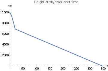
We might also want to check that they decelerate, so we can plot the velocity too:
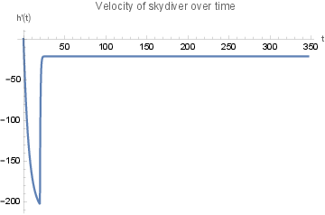
The two plots above were made using the following code:
Plot[First[h /. soln][t], {t, 0, tmax},
 PlotLabel -> "Height of skydiver over time",
 AxesLabel -> {"t", "h(t)"}]
and
Plot[First[h /. soln]'[t], {t, 0, tmax}, PlotRange -> Full,
 PlotLabel -> "Velocity of skydiver over time",
 AxesLabel -> {"t", "h'(t)"}]
Let’s unpack the solution a bit. Before, r was just a constant, but now we want to make it a function of time since it will change at some point. Thus, we change our equation from eqn = {h''[t] == -g - r*h'[t]} to eqn = {h''[t] == -g - r[t]*h'[t]};. We also add the option DiscreteVariables -> {r} in the call to NDSolve.
The way I have organized it, we don’t have to change anything with conds because those are just the initial conditions that force the rest of problem. Here is a nice time to point out that Mathematica will take care of figuring out the initial conditions for the “second” initial value problem we wanted to solve, namely the one after the parachute is deployed.
Now since r is a function of time we need to specify more information about it. We do this by giving the value r[0]==rFree of r when the skydiver is in freefall.
We also specify the event of parachute deployment by adding WhenEvent[t == 20, r[t] -> rChute]. This means that at 20 seconds, the parachute will be deployed.
Printing the value of tmax, we see that the ride now takes 346 seconds.
I think our skydiver will feel much better about this. We can get the speed at which they land by plugging in the value of tmax to the solution
First[h /. soln]'[tmax]
-21.3333
and we find that they hit the ground at a speed of a bit faster than 21 ft per second. Based on Human survivability of extreme impacts in free-fall (Snyder 1963) I think it is likely that our skydiver would be just fine.
A more realistic deployment
The US Parachute Association has a guideline that the parachutes should be deployed above somewhere between 2000 and 4500 feet above ground level depending on the skydivers experience. If we have a very experienced skydiver, lets have them jump not at around 7000 feet, but closer to 2000. We can do this by changing our WhenEvent. We’ll also want to know time at which the parachute is deployed, so we can throw a new variable tchute in to record the time at which the parachute is actually deployed. This code is
g = 32;
rFree = 0.15;
rChute = 1.5;
h0 = 10000;
eqn = {h''[t] == -g - r[t]*h'[t]};
conds = {h[0] == h0, h'[0] == 0};
events = {r[0] == rFree,
   WhenEvent[h[t] == 2000, tchute = t; r[t] -> rChute],
   WhenEvent[h[t] <= 0, tmax = t; "StopIntegration"]};
soln = NDSolve[{eqn, conds, events}, h, {t, 0, Infinity},
   DiscreteVariables -> {r}];
Plot[First[h /. soln][t], {t, 0, tmax},
 PlotLabel -> "Height of experienced skydiver over time",
 AxesLabel -> {"t", "h(t)"}]
Plot[First[h /. soln]'[t], {t, 0, tmax}, PlotRange -> Full,
 PlotLabel -> "Velocity of experienced skydiver over time",
 AxesLabel -> {"t", "h'(t)"}]
which gives us the plots
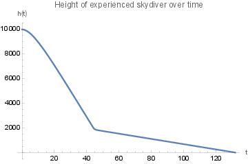
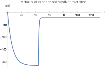
and we can see that the total jump takes around 132 seconds, with parachute deployment occuring at 44 seconds.