An example of the geometry of a combinatorial geometry
About a month ago, Dr. Federico Ardila dropped a survey paper entitled The Geometry of Geometries, surveying new and old aspects of matroid theory. I have been on a kick lately of really enjoying content he has written and also got the opportunity to chat with fellow graduate student Anastasia Nathanson about part of the paper. Dr. Galen Dorpalen-Barry taught me the value of a good example while she was a graduate student, so here is a little write up of the example which Anastasia and I came up with. Hopefully this is as helpful to you as it was to me in understanding section 4.1 of Ardila’s paper.
The Grassmannian
The complex Grassmannian \(\operatorname{Gr}(r,n)\) is a space whose points consists of \(r\)-dimensional subspaces of \(\mathbb{C}^n\). When I first heard about the Grassmannian I had lots of trouble picturing exactly what it should look like. Eventually I stopped trying to picture it and just took for granted that each point in the space is just a point in the space endowed with some extra meaning. So far that has helped me stop trying to think about it intuitively and instead just use my intuition as a point in topological space.
So lets pick a point \(x \in \operatorname{Gr}(2,4)\). It is a two-dimensional subspace of \(\mathbb{C}^4\). I can think of it as the span of two vectors in the (complex) vector space \(\mathbb{C}^4\). Suppose that \(x\) is the span of the vectors \((1, 0, -1, 0)\) and \((0, 1, 1, 0)\). Then I can represent the point \(x\) by the matrix \[ M = \begin{bmatrix} 1 & 0 & -1 & 0 \\ 0 & 1 & 1 & 0 \end{bmatrix}.\] If you like thinking of points spaces in terms of coordinates, you could think of this as a set of coordinates. But the one tricky thing is that there are multiple coordinates for a single point on the Grassmannian. For example, another coordinate for the same point is \[ \begin{bmatrix} -i & 0 & i & 0 \\ 0 & i & i & 0 \end{bmatrix}.\] (where \(i = \sqrt{-1}\)), because the row-space of \(M\) contains \(-i\) times the first row and \(i\) times the second row. The way I like to think of this is analogously to the “multiple coordinates for the same point” problem of polar coordinates. If you are familiar with polar coordinates, you’ll see that \((r, \theta) = (\sqrt{2}, \frac \pi 2) = (-\sqrt{2}, \frac{3\pi}{2})\). There is nothing wrong with these two coordinates giving the same point in space, just like there is nothing wrong with the two different matrices we gave to describe \(x\).
The general statement hiding in here is that a point in \(\operatorname{Gr}(r,n)\) can be given by an \(r \times n\) matrix. I should be careful and say that the rank of a matrix is the dimension of its row-space, so if I genuinely want a point of \(\operatorname{Gr}(r,n)\), then my \(r\times n\) matrix should have full rank.
Complex projective space
When \(r = 1\), the Grassmannian \(\operatorname{Gr}(1,n)\) goes by a special name - projective space. Projective space identifies all points up to a scalar. For example, the point \((1,2)\) and the point \((\frac 12, 1)\) are two different coordinates for the same \(\mathbb{C}^2\)-subspace/point in \(\operatorname{Gr}(1,2)\). (If you wish to think of it as a matrix, you should take the transpose of the two vectors I just gave.) If the first coordinates of \((x_1, x_2) \in \operatorname{Gr}(1,n)\) is not zero, then we can multiply by \(x_1^{-1}\) to get a point whose first coordinate is \(1\). Then we have one degree of freedom in the space, namely the choice of \(x_2\). This means that \(\operatorname{Gr}(1,2)\) is one-dimensional projective space: \(\mathbb{CP}^1\).
More generally, this phenomenon means that \(\operatorname{Gr}(1,n)\) is an \(n-1\)-dimensional manifold (a choice of local chart can be given by asserting that the \(i\)th coordinate is nonzero for \(1 \leq i \leq n\)). Given a point in the \((x_1, x_2) \in \mathbb{CP}^1\), we can think of it as going through \(\mathbb{C}^2\) first, before identifying all points in a common subspace. Following this pattern, we can include points in the Grassmannian \(\operatorname{Gr}(r,n)\) into \(\mathbb{CP}^{\binom{n}{r}-1}\) via the so-called “Plücker embedding.” The Plücker embedding takes the determinant of all full-rank submatrices of an \(r \times n\) matrix, and sets them to be coordinates in \(\mathbb{C}^{\binom{n}{r}}\). This is the right space because in order to take the determinant of full-rank submatrix it must be full-rank, and square. Thus, it should be the determinant of an \(r \times r\) matrix. Since we already have the \(r\)-many rows determined, picking an \(r\times r\) submatrix corresponds to picking \(r\) (out of \(n\) available) columns. Then by identifying points who differ only by a scalar, we drop the dimension by one as above to get a point in \(\mathbb{CP}^{\binom{n}{r}-1}\), from a point in \(\mathbb{C}^{\binom{n}{r}}\).
Lets see this process play out with the example of the matrix \(M\) above. Let $M_{i,j}$ denote the square matrix with all rows of \(M\) and the \(i\)th and \(j\)th columns.
| Columns \(i,j\) | \(\operatorname{det}(M_{i,j})\) |
|---|---|
| \(1,2\) | \(1\) |
| \(1,3\) | \(1\) |
| \(1,4\) | \(0\) |
| \(2,3\) | \(1\) |
| \(2,4\) | \(0\) |
| \(3,4\) | \(0\) |
So we get that the corresponding vector in \(\mathbb{C}^{\binom{n}{r}}\) is \((1,1,0,1,0,0)\). A few other ways to represend the corresponding point in \(\mathbb{CP}^5\) are as \((\frac{1}{2},\frac{1}{2},0,\frac{1}{2},0,0)\) or \((2,2,0,2,0,0)\).
Ardila writes the Plücker embedding as the map \(p\) and notes that “the map \(p\) provides a realization of the Grassmannian as a smooth projective variety.” I’m hoping to be able to write more about projective varieties in the future, but for now, the takeaway is that this is a nice embedding of the Grassmannian into a projective space.
Linear matroids
Now lets change gears from an geometric object corresponding to a matrices to a combinatorial object corresponding to a single matrix. Given a matrix, we can ask the question “which sets of column vectors are linearly independent”? While at surface level this might seem like a sort of boring, naive question, it turns out that this provides a level of generality to the situation which is quite incredible.
One way to describe a matroid is by defining the independent sets.
Def. A matroid \(M\) is a pair of a set \(E\) called the groundset with a collection \(\mathcal{I} \subset 2^E\) of elements satisfying the following conditions:
- The empty set is independent: \(\emptyset \in \mathcal{I}\)
- If \(A \in \mathcal{I}\) and \(B \subseteq A\), then \(B \in \mathcal{I}\)
- If \(A,B \in \mathcal{I}\) and \(|A| > |B|\), then there exists \(x \in A-B\) such that \(B \cup \{x\} \in \mathcal{I}\).
The intuition comes from the idea that the groundset \(E\) should be a set of vectors, and elements of \(\mathcal{I}\) should correspond to sets of vectors which are linearly independent. Indeed, taking the set of columns of a matrix together with the data of their linear indepdence defines a matroid, which is called a linear matroid.
Lets take a look at the matroid which comes from our matrix \[ M = \begin{bmatrix} 1 & 0 & -1 & 0 \\ 0 & 1 & 1 & 0 \end{bmatrix}.\] The set of vectors (from left to right) are \(a = \begin{bmatrix} 1\\0\end{bmatrix}\), \(b = \begin{bmatrix} 0\\1\end{bmatrix}\), \(c = \begin{bmatrix} -1\\1\end{bmatrix}\), \(d = \begin{bmatrix} 0\\0\end{bmatrix}\). Since \(d\), the zero vector, can’t be linearly independent with any of the others, and any collection of three vectors must contain a dependence we see that the set of linearly independent vectors are
\[ \mathcal{I} = \{\emptyset, \{a\}, \{b\}, \{c\}, \{a,b\}, \{a,c\}, \{b,c\} \} . \]
We’ll use the data of the independent sets to define a geometric object, but before we do that, it is worth mentioning that the notion of “independence” can be extended quite a bit. For instance, it can be extended to the relationship of edges within a graph, but for the full story you should go ahead and read Ardila’s article.
Matroid polytopes
A polytope in \(\mathbb{R}^n\) is an intersection of half-spaces which is bounded. The data of a matroid will allow us to define a polytope called a matroid polytope. In this case, the polytope will come as the convex hull of several points.
Def. Let \((E,\mathcal{I})\) be a matroid. A maximal (with respect to containment) independent set \(B \in \mathcal{I}\) is called a basis. The set of all bases is written \(\mathcal{B}\).
The various bases of our running example \(M\) are: \(\{a,b\}, \{a,c\}, \{b,c\}\).
Now we may define the polytope of a matroid. The polytope lives inside of a real vector space whose basis can be indexed by the groundset. In the case of our running linear matroid example, since the matrix is \(2 \times 4\), the matroid has a size-four groundset and so our matroid polytope will live inside of \(\mathbb{R}^4\).
The polytope associated to a matroid is given as the convex hull of the points of the form \(\sum_{i \in B} e_i\) where \(B\) is a basis of \(M\). Since we have three bases of our running example linear matroid, there are three points whose convex hull forms the matroid polytope. Those three points have coordinates \((1,1,0,0)\) and \((1,0,1,0)\) and \((0,1,1,0)\).
Visualizing matroid polytopes
I always get spooked by trying to visualize polytopes in high dimensions. But fortunately there are sometimes nice ways to visualize their projection into a lower dimension. Before describing this method, lets draw analogies in low dimensions.
The convex hull of the two standard basis vectors in \(\mathbb{R}^2\) forms a one-dimensional set of points. We could also consider the convex hull of the points \((2,0)\), and \((0,2)\). This would be the set of all points in the first quadrant whose sum is \(2\) - this can be thought of as the hyperplane \(x_1 + x_2 = 2\). In particular I want to call attention to the fact that the point \((1,1)\) lies on this hyperplane, for the sake of the analogy.
Similarly, we can think of the convex hull of \((3,0,0),\, (0,3,0),\, (0,0,3)\) as points in the positive orthant whose coordinate sum is \(3\) - the hyperplane \(x_1 + x_2 + x_3 = 3\).
Note that both of the two convex hulls above were geometric simplexes.
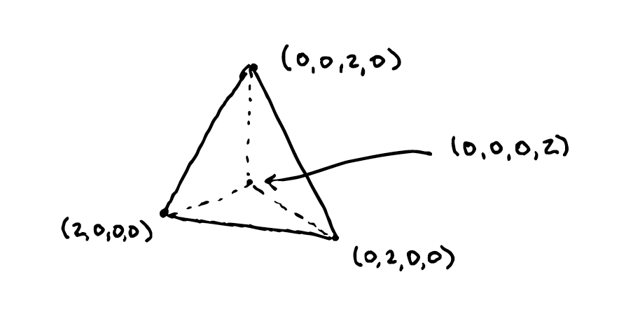
For our running example, we notice that we are taking the convex hull of points all of which have coordinate-sum \(2\), so we will want to consider them in the \(\mathbb{R}^4\)-hyperplane \(H\) defined by the equation \(x_1 + x_2 + x_3 + x_4 = 2\). The intersection of an affine hyperplane such as \(H\) with the positive orthant is, as we have hinted at already, a geometric simplex.
The geometric simplex in \(\mathbb{R}^4\) is a three-dimensional tetrahedron. Let us scale it by \(2\) so that each of its vertices correspond to points \((2,0,0,0)\), \((0,2,0,0)\), and so-on. Now we can draw the simplex.
Note that the midway points on each edge of the simplex have two coordinates equal to one, and two coordinates equal to zero:
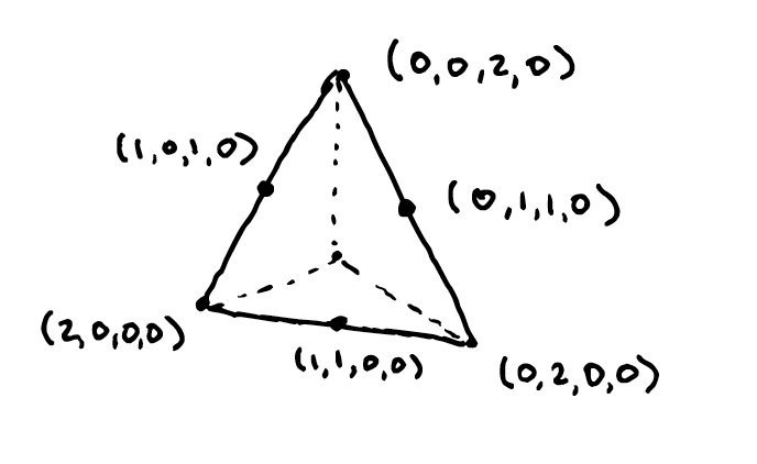
Three of the points matching this description are the vertices of our matroid polytope. Now we can draw their convex hull by restricting our attention to the simplex.
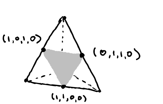
This process of restricting our attention to a scaled simplex is a nice way to visualize matroid polytopes which are a priori in \(\mathbb{R}^4\).
The image of some points
An amazing fact that, admittedly I don’t fully understand, draws the connection between the matroid polytope and the Grassmannian.
There is a map \(\mu: \operatorname{Gr}(r,n) \rightarrow \mathbb{R}^n\). Since I don’t fully understand the context behind the map, I’ll tell you what \(\mu\) is in a minute, but what this example taught me was the way that the “algebraic torus” \((\mathbb{C}^\star)^n\) (called a torus because it is homotopic to the topological torus \((S^1)^n\)) acts on a point in the Grassmannian.
Ardila writes that the torus “acts on the Grassmannian \(\operatorname{Gr}(r,n)\) by streching the \(n\) coordinate axes of \(\mathbb{C}^n\) modulo simultaneous streching.” I’m having trouble finding additional descriptions of this action but as best I can tell here is what it means: when we express a point \(V \in \operatorname{Gr}(r,n)\) in terms of coordinates, we can write a basis for \(V\) in terms of the standard basis of \(\mathbb{C}^n\). Then we take a vector \(\mathbf{x} \in (\mathbb{C}^\star)^n\) and multiply the standard basis vector \(e_1\) of \(\mathbb{C}^n\) by the first coordinate \(x_1\), and so on. The comment about “modulo simultaneous streching” is really referring to the fact that if \(\mathbf{y} = k \mathbf{x}\) for a scalar \(k\), then the action of \(\mathbf{y}\) and the action of \(\mathbf{x}\) upon a point \(V \in \operatorname{Gr}(r,n)\) are the same. This is because while \(\mathbf{x}\) and \(\mathbf{y}\) may act differently on a fixed coordinate representation (that is, a matrix) of a point in the Grassmannian, after taking the rowspace of the matrix the points are the same.
Let us see what this means for our running example. Consider \(\mathbf{x} = (2,3,-1,2)\) in the torus. I could have equally well chosen the points \((1,\frac32,\frac{-1}{2},1)\) or \((\frac23,1,\frac{-1}{3},\frac{2}{3})\), since we are working modulo simultaneous streching. Now, we want to act on the matrix \[ M = \begin{bmatrix} 1 & 0 & -1 & 0 \\ 0 & 1 & 1 & 0 \end{bmatrix}.\] Since we double the first coordinate, triple the second, negate the third, and double the fourth, we have that \[ \mathbf{x} \cdot M = \begin{bmatrix} 2 & 0 & 1 & 0 \\ 0 & 3 & -1 & 0 \end{bmatrix}.\] Notice that this is a genuinely different point in the Grassmannian, which we could write as \[ \mathbf{x} \cdot M = \begin{bmatrix} 1 & 0 & 1/2 & 0 \\ 0 & 1 & -1/3 & 0 \end{bmatrix}.\] We could also see that it is a genuinely different point by looking at its Plücker embedding in \(\mathbb{CP}^5\), which is \((1, \frac{-1}{3}, 0, \frac{-1}{2}, 0, 0) \neq k(1, 1, 0, 1, 0, 0)\).
Now we can define the map \(\mu: \operatorname{Gr}(r,n) \rightarrow \mathbb{R}^n\). Let \(V \in \operatorname{Gr}(r,n)\) and identify it with a matrix \(A\) whose rowspace is \(V\). Let \(B\) range over \(r\)-subsets of the columns of \(V\). Let \(A_{B}\) denote the \(r \times r\) submatrix of \(V\) which contains the columns of \(B\). Let \(e_B\) denote the sum of standard basis vectors in \(\mathbb{C}^n\) corresponding to the columns of \(B\). For example, if \(B\) consisted of the first, third, and seventh columns of a matrix, then \(e_B = e_1 + e_3 + e_7\). The map \(\mu\) is defined by \[ \mu(V) = \frac{\sum_B|\det A_B |^2 e_B}{\sum_B |\det A_B |^2}.\]
Now lets come back to our running example (and abuse notation identifying the matrix with its rowspace). We have \[ \mu(M) = \frac{1}{3} \left((1,1,0,0) + (1,0,1,0) + (0,1,1,0)\right) = \left(\frac{2}{3}, \frac{2}{3}, \frac{2}{3} \right)\] and \[ \mu( \mathbf{x} \cdot M) = \frac{1}{14} \left( (1,1,0,0) + 9(1,0,1,0) + 4(0,1,1,0) \right) = \left( \frac{5}{7}, \frac{5}{14}, \frac{13}{14}, 0 \right ).\]
Let us draw those points on the matroid polytope:
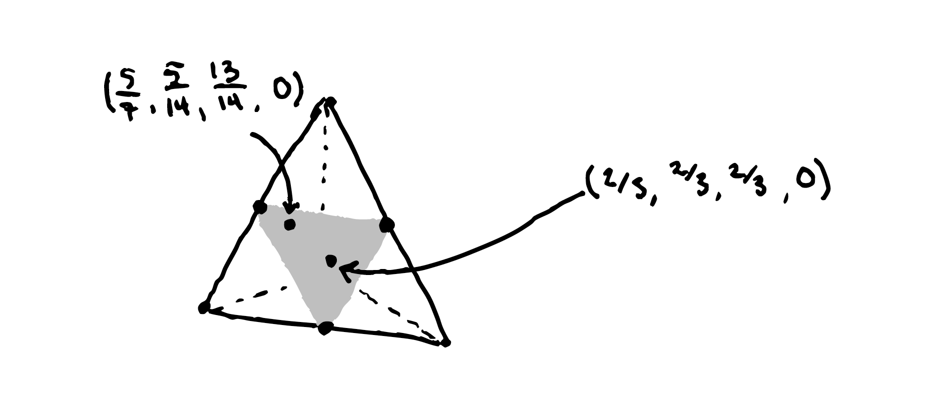
It is no coincidence that these points live on the matroid polytope. As Ardila points out, this is a theorem of Gelfand, Goresky, MacPherson, and Serganova that the closure of the torus-orbit of a point in the Grassmannian has \(\mu\)-image given by the matroid polytope. I find this fact incredible, and I hope you do too.